That distinction matters whenever a smooth return series becomes an allocation input. Lower measured volatility earns a larger position. A reassuring correlation earns a diversification label. Both can be influenced by the way prices arrive.
The fast price and the slow price
There is a real example in the BIS's 2024 Annual Economic Report. Exchange-traded real estate investment trusts and periodically appraised open-end property funds had diverged. The BIS interpreted the gap as a warning that commercial property losses could remain unrecognised elsewhere in the financial system. In the same chapter, it described infrequent valuation as a source of smoothed private-credit volatility. BIS, Chapter I.
The property comparison needs care. Listed and unlisted vehicles have different leverage, holdings and investors. Their prices cannot be treated as two interchangeable quotes for the same building. What the comparison exposes is a timing problem: a traded price can incorporate changed financing conditions before an appraisal catches up.
A portfolio risk model encounters that problem as data. It receives two return series with dates printed on them and treats those dates as comparable. One series may already reflect the shock. Another may distribute its recognition across several quarters. The covariance matrix inherits the difference.
In The One-Factor Portfolio, I argued that different asset labels can conceal a common exposure. Valuation timing adds another complication: even a return-based test for that exposure can be affected by the measurement process.
The uncertain number in the denominator
Unsmoothing has a long history. David Geltner's work on appraisal-based property returns and Getmansky, Lo and Makarov's research on hedge funds are foundations. A June 2026 working paper by Hoyeon Kang already applies the approach to private credit. The calculation here examines the resulting allocation sensitivity.
I used the public cumulative-return table for the Cliffwater Direct Lending Index, or CDLI. It measures unlevered, gross-of-fee loan-asset performance. It launched on 30 September 2015, with a reconstructed history beginning on 30 September 2004. These are asset returns, before the fees and financing of a particular investor's fund. Cliffwater's index factsheet.
The exercise starts with 87 quarterly returns, from the fourth quarter of 2004 through the second quarter of 2026. Regress each return on its predecessor, with an intercept, and the lag coefficient is 0.295. Use only the post-launch history and it falls to 0.107. That difference is central to the result.
Under a simple one-lag smoothing model, the inverse adjustment is rₜᵘ = (rₜ − α·rₜ₋₁)/(1 − α).
The assumption is that the reported return combines a current economic return with persistence from the previous mark. Attributing the fitted persistence to that mechanism is a modelling choice. Floating-rate income, genuine credit dynamics and changes in index composition can also create persistence. The adjustment cannot identify their individual contributions.
After dropping the first return needed as a lag, there are 86 matched quarters. I hold the adjusted series' arithmetic mean equal to the reported series' mean, then compare both with US equity returns and the cash benchmark from the Kenneth French Data Library.
| Measure | Reported | α = 0.107 | α = 0.295 |
|---|---|---|---|
| Annualised volatility | 3.31% | 3.61% | 4.48% |
| Conventional annualised Sharpe | 2.19 | 2.01 | 1.63 |
| Equity beta | 0.136 | 0.150 | 0.182 |
| Equity correlation | 0.670 | 0.674 | 0.661 |
The full-sample adjustment raises volatility by about 36%. The post-launch coefficient raises it by about 9%. The same reported history can therefore supply materially different risk inputs depending on the estimation window. These are sensitivity scenarios, rather than a statistical confidence interval. The split also crosses different credit regimes and index compositions; it does not establish that the valuation process itself changed at launch.
There is a separate check on beta. A Dimson-style regression of reported excess returns on current and previous-quarter equity excess returns gives coefficients summing to 0.176, close to the AR(1)-adjusted 0.182. Adding one leading quarter gives 0.203. This check avoids specifying an AR(1) smoothing coefficient, but still depends on which leads and lags enter the regression. The results are consistent with delayed co-movement; they do not identify its cause.
Correlation barely moves. A higher covariance need not produce a higher correlation when the adjusted series' own volatility also rises. The standalone Sharpe, meanwhile, is directly exposed to the volatility estimate: twice the quarterly mean excess return divided by its standard deviation. Holding the mean fixed takes the conventional annualised ratio from 2.19 to 1.63 under the full-sample adjustment. Serial dependence complicates square-root annualisation, so these are comparisons of conventional statistics, rather than measured one-year holding-period Sharpes.
Fees are of comparable importance. The annualised arithmetic mean excess return here is 7.47%. Subtracting an illustrative flat fund-level drag of 1.5–2 percentage points a year, while holding volatility fixed, lowers the reported-series Sharpe to approximately 1.75–1.60. Gross and net performance deserve the same care as reported and adjusted volatility.
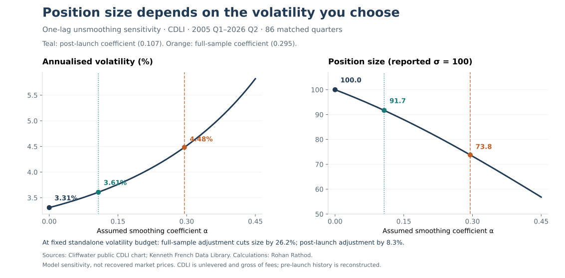
Now put the volatility estimate into a position-sizing rule. For a sleeve assigned a fixed standalone volatility budget, position size is proportional to 1/σ. Raising the input from 3.31% to 4.48% cuts the position to 73.8% of its previous size, a reduction of about 26%. Using 3.61% instead leaves it at 91.7%, a reduction of about 8%.
These are relative position sizes, not suggested portfolio allocations. A whole-portfolio volatility target would also depend on covariances and constraints. The mechanism is nevertheless clear: uncertainty about how returns are measured becomes uncertainty about how much capital the risk budget permits.
Whose risk is understated?
A genuinely locked-up investor has a strong objection. If liabilities are matched, leverage is absent and loans can be held through repayment or restructuring, a hypothetical sale price may have limited relevance to the decision. Covenants, seniority and lender control can improve outcomes. A smooth series alone cannot establish concealed losses or poor underwriting.
The FSB's May 2026 report acknowledges protective loan features and the ability of closed-end structures to limit liquidity mismatch. It also identifies the growth of vehicles offering redemption options and the incentive that stale valuations can create to leave before a markdown. FSB, Report on Vulnerabilities in Private Credit, sections 3.3 and 4.
Consider a simplified fund with assets economically worth 90 and a reported NAV of 100. An investor owning 10% can redeem for 10 before the valuation changes. Before that redemption, the remaining investors' 90% share was economically worth 81. Afterwards, they hold 80. The departing investor took one unit from them. This illustration assumes sufficient cash and no adjustment to the redemption price; actual dealing terms can change the outcome.
Lockups, gates and valuation updates can restrict that transfer. They also define which risk belongs to whom. The investor seeking an exit bears access risk. Remaining investors face potential dilution. A leveraged holder may have cash obligations before the underlying loans repay. A risk budget built from quarterly NAVs needs to account for those different horizons.
The relevant question is whether the investor's cash needs and contractual obligations permit the patience that the asset requires.
What belongs beside the ratio
A useful risk report should show:
- The valuation date, update frequency and age of each material mark.
- Reported volatility and sensitivity to plausible valuation lags.
- Borrower exposures, covenant protection and stressed recoveries.
- Redemption terms, collateral obligations and assets available to meet cash demands.
The attractive Sharpe may partly describe the investment. It may also partly describe the reporting process. An allocation decision needs to know how much it depends on each.
Reproducibility note. Calculations, source links and chart files are in the accompanying research notes. The exercise uses the full sample for descriptive estimation, not a historical trading rule. The adjusted series is a model sensitivity estimate; it is not an observed transaction-price series. All allocation comparisons use the same matched sample and unchanged mean return.
Research notes and downloads
Source observations were captured on 30 October 2026. The main comparison uses 86 matched quarters, 2005 Q1–2026 Q2. CDLI data end in June 2026.
Downloads
- Calculation results (JSON)
- Python analysis — requires NumPy, pandas and Matplotlib.
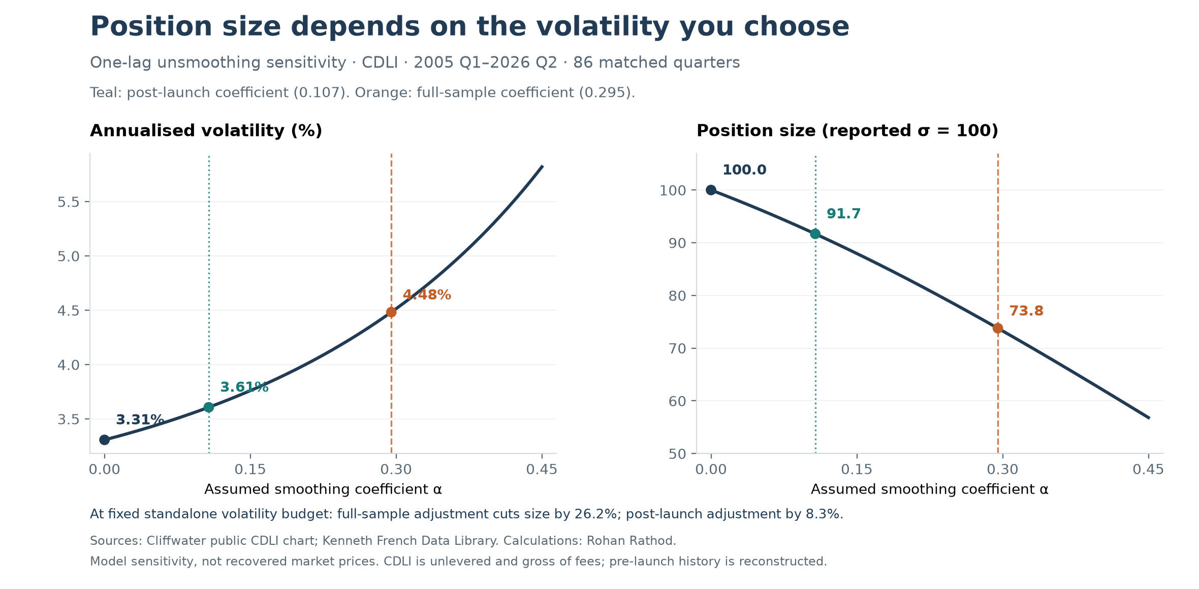
- Chart (SVG) · Chart (PNG)
Reproduce the calculations
- Open the public CDLI chart, select “View as data table” under “CDLI Cumulative Returns by Component”, and save the displayed table as
cdli-public-chart.tsv, retaining dates from 30 September 2004 through 30 June 2026. The snapshot used here contains 88 cumulative quarterly levels; the calculations use the total-return column. - Download the monthly Fama/French three-factor CSV, extract it and save it as
fama-french-factors-source.csv. These results use the September 2026 CRSP vintage. Later releases may revise historical values; input hashes are included in the results file. - Save the analysis download as
analyse.pybeside those two inputs and runpython analyse.py. The script makes no network requests and writes the results, matched observations and chart files.
Definitions and assumptions
- Quarterly CDLI returns are changes in adjacent cumulative total-return levels. The full-sample AR(1) fit has an intercept and 86 lag pairs. The post-launch fit uses 42 pairs entirely within 2015 Q4–2026 Q2.
- The one-lag inverse is recentered to preserve the matched sample’s arithmetic mean. It does not preserve compounded wealth or identify transaction prices.
- Monthly US equity total returns are
Mkt-RF + RFfrom the Kenneth French Data Library. Monthly equity and cash returns are compounded separately into quarters. The benchmark is the broad US CRSP market. - Volatility is quarterly total-return sample standard deviation × 2. Conventional Sharpe is quarterly mean excess return / excess-return standard deviation × 2. The cash return varies, so the two standard deviations differ. Neither statistic is adjusted for serial dependence across a one-year holding period.
- Beta uses excess returns and an intercept; correlation uses total returns. The current-plus-one-lag beta is 0.176303, with a Newey–West standard error of 0.032172 using two quarterly lags. Adding one lead gives 0.203330 on the same 86 quarters; the two-lag variant gives 0.205182 on 85 quarters. The lead check uses 2026 Q3 market observations available in the source vintage.
- Relative position size at a fixed standalone volatility budget is reported σ / adjusted σ. Whole-portfolio sizing also depends on covariances and constraints. Earlier two-asset equal-risk-budget diagnostics remain in the results file for completeness.
- The fee illustration subtracts a constant annual return drag divided by four from quarterly returns. It is not an estimate of a particular fund’s fee schedule or financing costs.
The model is a descriptive sensitivity test. Persistence may reflect income dynamics, credit conditions, valuation mechanics or changing composition. Full-sample estimation is not a historical trading rule. Differences between estimation windows do not establish a structural break at index launch.
Rohan Rathod, London, October 2026